Cost Analysis Techniques

As noted earlier, more and more organizations are shifting their attention away from price management and toward cost management. In so doing, there may be opportunities to reduce costs that are not available when the discussion focuses only on price. In cost analysis, the supply manager performs a detailed analysis of the different elements of costs shown earlier in Exhibit 11.6 and identifies what is driving the different elements.

Cost-Based Pricing Models

Cost Markup Pricing Model

In this model, the supplier simply takes its estimate of costs and adds a markup percentage to obtain the desired profit. This markup percentage could be added to the product cost only (usually direct materials plus direct labor plus production overhead), in which case the markup would have to provide for profit, plus all other indirect costs of operating the business. However, if the markup is applied to the total cost (product cost plus general, administrative, and sales expenses), then the markup is solely profit to the supplier. For example, a supplier that wanted a 20 percent markup over its total cost of $50 would quote a price of $60 ($50 + (20% of $50) = $60), which would leave a profit of $10.

Margin Pricing Model

In the margin pricing model, the supplier is still attempting to obtain a profit related to its costs, but instead of adding a markup to cost, the supplier establishes a price that will provide a profit margin that is a predetermined percentage of the quoted price (i.e., not a percentage of cost, as in markup pricing). For example, the supplier discovered that last year its margin as a percentage of sales was 1 percent, and this year the supplier would like it to be 20 percent. Using the same total cost of $50 as above would result in the supplier quoting a price of $62.50 in order to obtain the margin of 20 percent. This is calculated using the new equation for margin pricing:

Cost + ðMargin Rate × Unit Selling PriceÞ = Unit Selling Price

Using simple algebra, solving the equation for unit selling price results in the formula:

Cost=ð1 − Margin RateÞ = Unit Selling Price

or

ð$50Þ=ð1 − 20%Þ = Unit Selling Price

As in cost markup pricing, the supply manager must be aware if the margin pricing is based on product cost only or if it is based on total cost.

Rate-of-Return Pricing Model

A third common model in the cost-based category is the rate-of-return pricing model, wherein the desired profit is added to the estimated cost. In this model, the supplier bases the profit on the objective of a specific desired return on the financial investment, rather than on the estimated cost. For example, if the supplier wanted a 20 percent re- turn on its investment of $300,000 (which might include R&D, equipment, engineering, or other elements), to make 4,000 parts with a total cost of $50 each, the quoted price would be $65, using the following approach:

Unit Cost + Unit Profit = Unit Selling Price

$50 + ðð20% × 300; 000Þ=4;000Þ = $65

Product Specifications

Whether they realize it or not, purchasers impact price at the time they set the speci- fications for the product or service. Specifying products or services requiring custom design and tooling affects a seller’s price, which is one of the reasons purchasers try to specify industry-standard parts whenever possible. Cost (and hence price) becomes higher as firms increase the value-added requirements for an item through design, tool- ing, or engineering requirements. Purchasers should specify industry-accepted standard parts for as much of their component requirements as possible and rely on customized items when they provide a competitive product advantage or help differentiate a product in the marketplace.

The ability to perform a cost analysis is a direct function of the quality and availability of information. If a purchaser and seller maintain a distant relationship, cost data will be more difficult to identify due to the lack of support from the seller. An obvious approach that can help in obtaining necessary cost data is to require a detailed production cost breakdown when a seller submits a purchase quotation. The reliability of self-reported cost data must be considered. Another approach or option involves the joint sharing of cost information. A cross-functional team composed of engineers and manufacturing personnel from both companies may meet to identify potential areas of the supplier’s process (or the purchaser’s requirements) that can potentially reduce costs. One of the benefits of developing closer relations with key suppliers is the increased visibility of sup- plier cost data. The following section details some techniques that focus on cost.

Estimating Supplier Costs Using Reverse Price Analysis

Often suppliers will not be forthcoming in sharing cost data. In these situations, the purchaser must resort to a different type of analytical approach called “reverse price analysis” (also known as “should cost” analysis). A seller’s cost structure affects price be- cause, in the long run, the seller must price at a level that covers all variable costs of production, contributes to some portion of fixed costs, and contributes to some level of profit. As discussed later in the chapter, many suppliers are reluctant to share internal cost information. This information, however, is valuable to a purchaser, particularly when evaluating whether a supplier’s price is justifiable and reasonable. In the absence of specific cost data, a supplier’s overall cost structure must be estimated using a cost analysis—meaning that if the supplier is assigning costs in an appropriate manner, what should the product cost based on these calculations?

Information about a specific product or product line is often difficult to identify. A purchaser may have to use internal engineering estimates about what it costs to produce an item, rely on historical experience and judgment to estimate costs, or review public financial documents to identify key cost data about the seller. The latter approach works best with publicly traded small suppliers producing limited product lines. Financial documents allow estimation of a supplier’s overall cost structure. The drawback is that these documents do not provide much information about a specific breakdown of cost by product or product line. Also, if a supplier is a privately held company, cost data be- come difficult to obtain or estimate.

Despite these difficulties, there are tools available that can be used to estimate a sup- plier’s cost using some publicly available information. When evaluating a supplier’s costs, the major determinants of a supplier’s total cost structure must be taken into consider- ation. Let’s assume a supply management manager is buying a product or service for the first time without experience of what fair pricing might be. Because they do not have the tools at hand, or because they are too busy, many purchasers’ usual technique is to go with their gut feel or to evaluate competitive bids. It may be worth the time and effort, however, to perform some additional research using data from an income statement or from Internet sites. In doing so, the purchaser may perform a reverse price analysis— which essentially means breaking down the price into its components of material, labor, overhead, and profit.

Let’s start the process with a supplier-provided price of $20 per unit. The first com- ponent to consider is the price contribution toward profit, and sales, general, and admin- istrative (SGA) expenses. For publicly traded companies, this can be estimated by looking at a variety of websites that provide information on financial reports, including balance sheets, income statements, cash flow statements, and annual reports shown in Exhibit 11.11 under the “Financial Reports” section.

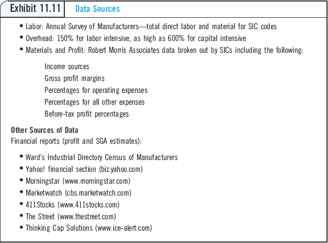
Exhibit 11.11 provides a list of available data sources for other components of cost. For this example, assume the purchaser determined that the supplier is a privately held com- pany. This is still not a problem, assuming the buyer can look up the supplier’s SIC code (www.FreeEDGAR.com). Another useful resource is Robert Morris Association (www. rmahq.org), which publishes the gross profit margin for this SIC overall, as well as before- tax profit percentages. Although this is a rough estimate, it does offer a good starting point. In Exhibit 11.12, the gross profit and SGA expense percentage for this supplier’s SIC code is 15 percent. Thus, on a price of $20, the estimated profit is $3. Next, the purchaser will need to understand the labor and material cost components of price.

Material costs can often be estimated by consulting with internal engineers. Using an estimate of required material, as well as external information on current pricing of these materials (as shown in the previous section), a rough estimate can be made of the amount of material in the product. In our example, we discovered that an approximation of the amount of material included is 20 percent of the price, or $4.

To find out how much labor is included, the best place to look is the Annual Survey of Manufacturers, published by the U.S. Department of Commerce and available at http://www.census.gov/prod/www/abs/industry.html. This site allows the purchaser to download information on total direct-labor costs and total material costs for any SIC number. This information allows the purchaser to calculate a materials-to-labor ratio. For the analysis shown in Exhibit 11.12, suppose that the purchaser discovered that the ratio of materials to labor based on the SIC code was 1.333. Thus, if material costs were previously estimated at $4, then direct-labor costs should be approximately $3 (4/1.333).

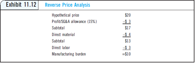
After subtracting the estimates for profit/SGA, materials, and labor from the price, the remaining portion of cost is considered manufacturing burden or overhead. At this point, the purchaser must determine whether $10 per unit paid on a price of $20 per unit is a reasonable amount for overhead costs. Typically, overhead is expressed as a per- centage of labor costs. For labor-intensive industries, the ratio could be as low as 150 percent. For capital-intensive industries, it could be as high as 600 percent. In our exam- ple, the overhead rate is 333 percent of labor ($10/$3). Using other data from Robert Morris Associates, the purchaser can also estimate the percentages for operating ex- penses and for all other expenses. With this cost estimate in hand, the purchaser should now be able to approach the supplier in a negotiation and initiate a discussion that ad- dresses price and cost. Although these estimates may not be 100 percent accurate, they provide a baseline for discussion of the supplier’s cost structure.

Labor cost will be an increasing factor in many cost estimates. The period from 2010 to 2015 will see the next impact of the baby boomer population on society. This impact will be in terms of a large number of people from this group retiring and leaving the work force. The number of retirees from multiple industries is expected to reach levels that have never been seen previously.

At the same time, the U.S. economy will continue to grow, and the demand for labor will escalate proportionately. Given the movement toward the service economy, the need for labor in selected industries is expected to grow significantly. Experts believe that ser- vices will be most affected, with a 29 percent growth rate. Transportation, retail trade, construction, and wholesale trade labor demand will also increase by double digits dur- ing this period. In construction alone, demand for drilling, specialty trades, and refining positions will increase by 17 to 18 percent during this period. In discussing the supplier’s cost structure with the supplier and how it applies to the price paid, the purchaser should attempt to initiate discussion in the following areas to discover opportunities for cost reductions.

• Plant utilization. The cost impact of additional business on the operating efficiency of a supplier should be evaluated. Is a supplier currently operating at capacity? Will additional volume actually create higher costs through overtime? Or will a supplier be able to reduce its cost structure through additional volume? The utilization rate of productive assets contributes directly to a supplier’s cost structure.

• Process capability. The purchaser should also consider if projected volume requirements match a supplier’s process capability. It may be inefficient to source smaller lot sizes with a supplier that requires long runs to minimize costs. On the other hand, suppliers specializing in smaller batches cannot effi- ciently accommodate volumes requiring longer production runs. A supplier’s production processes should match a purchaser’s production requirements. Supply management should also evaluate production processes to determine if they are state-of-the-art or rely on outdated technology. Production and process capability influences operating efficiencies, quality, and the overall cost structure of a seller.

• Learning-curve effect. Learning-curve analysis indicates whether a seller can lower its cost as a result of the repetitive production of an item.

• The supplier’s workforce. A supplier’s labor force affects the cost structure. Issues such as unionized versus nonunionized, motivated versus unmotivated, and the quality awareness and commitment of employees all combine to add another component to the cost structure. When visiting a supplier’s facility, representa- tives from the purchaser should take the time to talk with employees about quality and other work-related items. Meeting with employees provides valuable insight about a supplier’s operation. In recent years, the cost of labor in the workforce has gone up dramatically.

• Management capability. Management affects costs by directing the workforce in the most efficient manner, committing resources for longer-term productivity improvements, defining a firm’s quality requirements, managing technology, and assigning financial resources in an optimal manner. Management efficiency and capability have both a tangible and intangible impact on a firm’s cost structure. In the end, every cost component is a direct result of management action taken at some point in time.

• Supply management efficiency. How well suppliers purchase their goods and services has a direct impact on purchase price. Suppliers face many of the same uncertainties and forces in their supply markets that purchasers face. Supplier visits and evaluations should evaluate the tools and techniques suppliers use to meet their material requirements.

Break-Even Analysis

Break-even analysis includes both cost and revenue data for an item to identify the point where revenue equals cost, and the expected profit or loss at different production volumes.

Firms perform break-even analysis at different organizational levels. At the highest levels, top management uses this technique as a strategic planning tool. For example, an automobile manufacturer can use the tool to estimate expected profit or loss over a range of automobile sales. If the analysis indicates that the break-even point in units has risen over previous estimates, cost-cutting strategies can be put in place. Divisions or business units can use the technique to estimate the break-even point for a new prod- uct line.

Supply management and supply chain specialists use break-even analysis to develop the following insights:

• Identify if a target purchase price provides a reasonable profit to a supplier given the supplier’s cost structure.

• Analyze a supplier’s cost structure. Break-even analysis requires detailed analy- sis or estimation of the costs to produce an item.

• Perform sensitivity (what-if) analysis by evaluating the impact on a supplier of different mixes of purchase volumes and target purchase prices.

• Prepare for negotiation. Break-even analysis allows a purchaser to anticipate a seller’s pricing strategy during negotiations. Research indicates that a direct relationship exists between preparation and negotiating effectiveness.

Did BP Make a Total Cost Decision on the Deepwater Horizon?

BP PLC engineers made a series of cost-conscious decisions that ran counter to the advice of key contractors in the days leading up to the April 20, 2010 Deepwater Horizon rig explosion, accord- ing to documents released by a congressional panel.

“Time after time, it appears that BP made decisions that increased the risk of a blowout to save the company time or expense,” Reps. Henry Waxman (D., Calif.) and Bart Stupak (D., Mich.) wrote to Mr. Tony Hayward, CEO of BP. The two lawmakers are the top Democrats on the House Energy and Commerce Committee. In one case, BP engineers decided on April 16 to use just six so-called “centralizers” to stabilize the well before cementing it, instead of 21 as recommended by contractor Halliburton Corp. ac- cording to BP internal e-mails made public by the panel. In their letter, the lawmakers say that BP’s well team leader, John Guide, “raised objections to the use of the additional centralizers” in an April 16 e-mail released by the panel. “It will take 10 hrs to install them … I do not like this,” Mr. Guide wrote.

The explosion and fire aboard the Deepwater Horizon rig in the Gulf of Mexico triggered a spill estimated at 200M barrels. BP has created a $20B cleanup and relief fund to compensate for this problem. The lawmakers’ letter cited “five crucial decisions” BP made in designing and completing the well, which may have led to vulnerabilities in the well’s design. “The common feature of these five decisions is that they posed a trade-off between cost and well safety,” the letter says. Con- gressional investigators zeroed in on decisions by BP taken when drilling had ended, but work on temporarily shutting the well was still under way.

The most critical decision involved choosing the final piece of pipe for the well. BP opted for a “long string”—a pipe that runs all the way from the floor of the sea to the bottom of the well. In an internal BP e-mail from March 30, a BP drilling engineer in Houston told colleagues that this option “saves a good deal of time/money.” But it also created a direct pathway for gas and oil to rise up the backside of the well, a point recognized by a BP internal review from a few days be- fore the well blowout was not released by the congressional panel. The other option a so-called liner tieback—would have taken several days longer and cost more, but would have made the well more secure by adding new barriers to prevent gas from flowing unchecked toward the surface, according to the BP review. Using a liner would have cost an additional $7 million to $10 million, according to a BP estimate. Consider the savings that could have been generated from a total cost perspective if the other liner had been used!

While the liner option was costlier, internal BP documents suggest it was the safer choice. “Primary cement job has slightly higher chance” of setting correctly with a liner, notes a BP document from mid-April. After BP chose the long string, it made other time-saving choices that made the well more dangerous, Mr. Waxman and Mr. Stupak claim in their letter. Mr. Waxman also highlighted BP’s de- cision not to take 12 hours to completely circulate the heavy drilling fluid in the well, a step that would have allowed them to check if gas was leaking into the well and clean it out.

BP also skipped a test to determine if the cement had properly bonded to the well and rock for- mations, according to documents from oilfield service firm Schlumberger Ltd., whose crew was sent back to shore hours before the explosion. While the test would have allowed BP to check if the cement job was adequate and allowed for repairs, it would have taken nine to twelve hours just for the test. A petroleum engineer advising the congressional committee called the decision not to run a cement bond test “horribly negligent.”

Source: King, N., and Gold, R. (2010, June 15), “BP Focused on Costs: Congress,” Wall Street Journal, A1.

Sourcing Snapshot Measuring Supply Management’s Cost Savings at a Large Consumer Packaged Goods Company

A CPG company has $12B in controlled spend. Within this organization. however, there were several “rifts” that were occurring. Procurement had no credibility with senior management, due to the fact that the savings the team claimed to achieve were not credible and were not “believed” by other business stakeholders. Although Supply Management had indeed generated savings, these savings were being measured using Purchase Price Variance (PPV)—which simply measured the change in prices paid on an annual basis. PPV savings varied widely, based on market volatility and changes in market prices and, as a result, the Chief Financial Officer (CFO) challenged these savings as being invalid. The Chief Procurement Officer (CPO) felt that his team was generating benefits, but finance did not have a proper understanding of market volatility. Further, finance was not seen as an partner to procurement, and the CPO emphasized that the CFO did not understand long-term contracts.

In fact, the real problem in this case was the PPV metric, which was ineffective, unreliable, and could not be well communicated and translated to stakeholders. The metric drove questions such as “Did we overpay last year?,” “Should we have saved 30 percent instead of 10 percent?” and the like. And no one was sure of how to better align financial budgets to market realities. At this stage, the CEO became involved, as he possessed some procurement experience. His analogy to the PPV metric went something like this: “Investors have a portfolio, and our company is measured by our stock price relative to other companies in that portfolio. If it goes up 5 percent relative to a market that goes up by 10 percent, that is not good. But if the market shrinks by 10 percent and our share price is only down by 5 percent, analysts will buy our stock. So why can’t we establish a similar set of measurements for supply management performance? Can we create a portfolio to measure supply management price performance?” The CEO recommended to move to a market benchmarking basis where procurement had a Purchase Price Index that was measured against market indicators.

The next battle was how to measure market pricing? Benchmarking some categories such as true commodities was easy, as indicators existed for these items (e.g., paper, resin, and so forth). But there were also special commodities whose price behavior was more erratic. For this situation, the company hired a third-party market research provider, Beroe, to create a true commodity baseline and historical relationship, and then calculate an offset. For a finished product, Beroe created a cost driver model that calibrated company spend to market costs, and used market trends to define benchmarks. Savings performance moved from a project focus to a portfolio focus.

The next challenge? Procurement is also being asked to continue to monitor supplier financial risk and carbon footprint, and ensure integration with stakeholders. As procurement plays a more important role in the strategic planning of this organization, they are being tasked to be- come more creative in understanding risks and opportunities in the supply chain, and communicating these to stakeholders.

Source: Bucci, M. B. (December, 2009) Sales Director, Beroe, Inc., presentation, Supply Chain Resource Cooperative

Break-even analysis requires the purchaser to identify the important costs and revenues associated with a product or product line. Graphing the data presents a visual representation of the expected loss or profit at various production levels. Cost equations also express the expected relationship between cost, volume, and profit. When using break- even analysis, certain common assumptions are typically used:

1. Fixed costs remain constant over the period and volumes considered.

2. Variable costs fluctuate in a linear fashion, although this may not always be the case.

3. Revenues vary directly with volume. This is represented graphically by an upward-sloping total revenue line beginning at the origin.

4. The fixed and variable costs include the semivariable costs. Thus no semivariable cost line exists.

5. Break-even analysis considers total costs rather than average costs. However, the technique often uses the average selling price for an item to calculate the total revenue line.

6. Significant joint (i.e., shared) costs among departments or products limits the use of this technique if these costs cannot be reasonably apportioned among users. If shared costs cannot be apportioned, then break-even analysis is best suited for the entire operation versus individual departments, products, or product lines.

7. This technique considers only quantitative factors. If qualitative factors are important, management must consider these before making any decisions based on the break-even analysis.

Break-Even Analysis Example

The following example assumes that fixed costs, variable costs, and target purchase price for a single item are reasonably accurate. The construction of a break-even graph requires these three pieces of information.

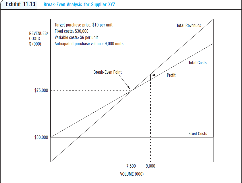
Exhibit 11.13 shows the required cost and volume data along with the break-even graph for this example. Because a buyer is estimating the break-even analysis for a supplier, the price is a target purchase price established by the purchaser. A range of prices can be analyzed to estimate a supplier’s expected profit or loss given the fixed and variable costs.

In this example, the purchaser wants to determine if the anticipated volume of 9,000 units provides an adequate profit for the supplier at the target purchase price.

Exhibit 11.13 indicates that the supplier requires at least 7,500 units to avoid a loss with this cost structure and target purchase price. The following equation identifies the profit or loss associated with a given volume:

Net Income or Loss = ðPÞðXÞ − ðVCÞðXÞ − ðFCÞ

where P = average purchase price, X = units produced, VC = variable cost per unit of production, and FC = fixed cost of production for an item.

The supplier’s expected profit for the anticipated 9,000 units is calculated as follows, using $10 per unit as the average purchase price:

Net Income = ð$10Þð9;000Þ − ð$6Þð9;000Þ − ð$30;000Þ= $60000 Profit

We can also calculate the number of units the supplier needs to produce to break even (i.e., cover fixed costs). This is calculated as follows:

Total Revenue = Variable Cost + Fixed Cost

$10ðXÞ = $6ðXÞ + $30;000

$4ðXÞ = $30;000

X = 75000 units

If the cost data are accurate, then the anticipated purchase volume provides a profit to the supplier, because it exceeds 7,500 units. Whether this is an acceptable profit level given the cost structure is an issue both parties may have to negotiate. If the analysis indicates that the purchase volume results in an expected loss to the seller, then a pur- chaser must consider several important questions:

• Is the target purchase price too optimistic given the supplier’s cost structure?

• Are the supplier’s production costs reasonable compared with other producers in the industry?

• Are the cost and volume estimates accurate?

• If the cost, volume, and target price are reasonable, is this the right supplier to produce this item?

• Will direct assistance help reduce costs at the supplier?

This method allows an evaluation of a supplier’s expected profit over a range of costs, volumes, and target purchase prices. The break-even technique, however, often provides only broad insight into a purchase decision.